Necessary R libraries
# Install, if necessary, and load necessary libraries and set up R session
#if (!requireNamespace("BiocManager", quietly = TRUE)) install.packages("BiocManager")
library(ggplot2)
library(ggfortify)
library(corral)
library(ade4)
library(irlba)
library(glmpca)
library(ggplot2)
library(scatterD3)
suppressPackageStartupMessages(library(ComplexHeatmap))
Background
Decomposition of the Pearson residuals is a excellent method for exploratory analysis of count data and is also know as correspondence analysis. Because of its speed (which is comparable to PCA) and its performance it has been adopted by many fields. Correspondence analysis was originally proposed in 1935 (Hirschfeld, 1935), and was later developed by Benzécri as part of the French duality diagram framework for multivariate statistics (Benzécri, 1973; Holmes, 2008). His trainee Michael Greenacre later popularized its use with large, sparse count data in diverse settings and disciplines, including linguistics, business and marketing research, and archaeology (Greenacre, 1984, 2010). In numerical ecology, it is commonly applied to analyzing species abundance count matrices (M. Greenacre, 2013; Legendre et al., 1998). It has been successfully applied to microarray transcriptomics data (Fellenberg et al., 2001). and a Bioconductor version was implemented in the made4 Bioconductor package by Culhane et al., (2002) and the method was also used in joint and multi-table factorization methods (Culhane et al., 2003; Meng et al., 2014). Its first application on single cell RNA seq was in analysis of metagenomic scRNAseq microbiome census data data (McMurdie & Holmes, 2013). Correspondence analysis is available in the ade4 and vegan R packages and was listed in a review of single and multi-table matrix factorization approaches (Meng C, Zeleznik OA. et al., 2016).
Correspondence analysis (COA) is considered a dual-scaling method, because both the rows and columns are scaled prior to singular value decomposition (SVD). Lauren Hsu provided a description of COA applied to both single and a multi-table extension to joint decomposition of single cell RNA seq in her master’s thesis (Biostatistics, Harvard School of Public Health, 2020) and has implemented a fast implementation of COA that supports sparse matrix operations and scalable svd (IRBLA) in her Bioconductor package corral.
Hafemeister and Satija in their characterization of the SCTransform method propose that Pearson residuals of a regularized negative binomial model (a generalized linear model with sequencing depth as a covariate) could be used to remove technical characteristics while preserving biological heterogeneity, with the residuals used directly as input for downstream analysis, in place of log-transformed counts (Hafemeister & Satija, 2019) In the Townes et al., (2019), generalized principal component analysis (GLM-PCA), a generalization of PCA to exponential family likelihoods but report that both the multinomial and Dirichlet-multinomial are computationally intractable on single cell data and propose Poisson and negative binomial likelihood models, and focusing on Poisson glmPCA due to its performance.
Single cell RNAseq data are counts and naturally Poisson, therefore the application of Pearson residuals by both Townes et al., (2019) and Hafemeister and Satija (2019) show how correspondence analysis has been “rediscovered.” In reviews by Abdi & Valentin, 2007; Greenacre, 2010, they remark how frequently COA is rediscovered but each rediscovery enforces its importance to the field
In this vignette we compare different approaches for applying COA in R.
Toy Dataset
The function simData() in the glmPCA vignette, orginally provided by Jake Yeung created a simulated dataset with 4989 rows and 150 columns, 3 biological groups (clusters) of 50 cells each and 2 batches. 5000 rows are created but some are filtered to create a matrix of 4989 rows.
simData<-function() {
    set.seed(202)
  ngenes <- 5000 #must be divisible by 10
  ngenes_informative<-ngenes*.1
  ncells <- 50 #number of cells per cluster, must be divisible by 2
  nclust<- 3
  # simulate two batches with different depths
  batch<-rep(1:2, each = nclust*ncells/2)
  ncounts <- rpois(ncells*nclust, lambda = 1000*batch)
  # generate profiles for 3 clusters
  profiles_informative <- replicate(nclust, exp(rnorm(ngenes_informative)))
  profiles_const<-matrix(ncol=nclust,rep(exp(rnorm(ngenes-ngenes_informative)),nclust))
  profiles <- rbind(profiles_informative,profiles_const)
  # generate cluster labels
  clust <- sample(rep(1:3, each = ncells))
  # generate single-cell transcriptomes
  counts <- sapply(seq_along(clust), function(i){
    rmultinom(1, ncounts[i], prob = profiles[,clust[i]])
  })
  rownames(counts) <- paste("gene", seq(nrow(counts)), sep = "_")
  colnames(counts) <- paste("cell", seq(ncol(counts)), sep = "_")
  # clean up rows
  Y <- counts[rowSums(counts) > 0, ]
  sz<-colSums(Y)
  Ycpm<-1e6*t(t(Y)/sz)
  Yl2<-log2(1+Ycpm)
  z<-log10(sz)
  pz<-1-colMeans(Y>0)
  cm<-data.frame(total_counts=sz,zero_frac=pz,clust=factor(clust),batch=factor(batch))
  return(list(Y=Y, pheno=cm))
}
simDataObj <-simData()
mat=simDataObj$Y
pheno=simDataObj$pheno
dim(mat)
## [1] 4989 150
dim(mat)## [1] 4989 150There are 3 clusters and 2 batches
table(pheno$clust, pheno$batch)##
## 1 2
## 1 27 23
## 2 25 25
## 3 23 27PCA of toy data (to enable comparison of methods)
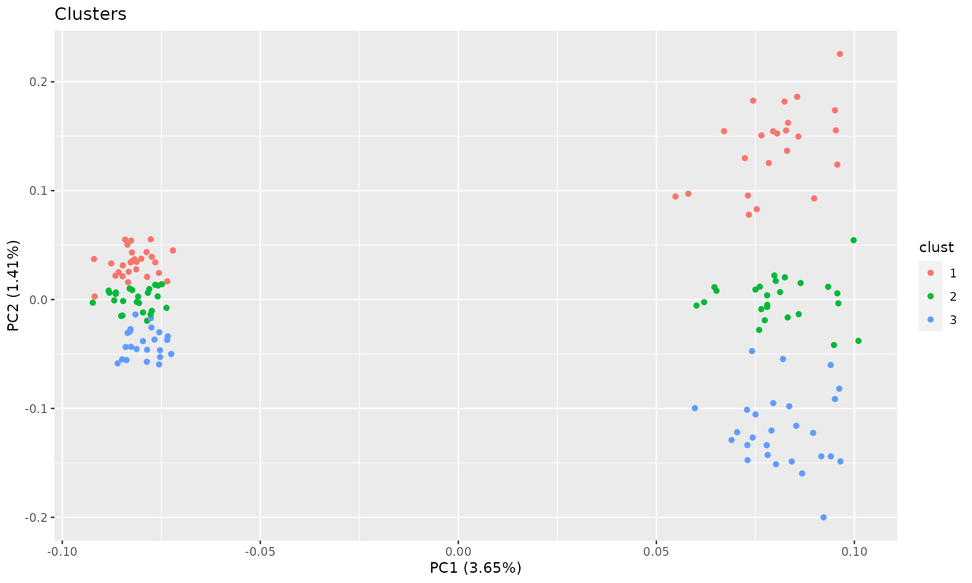
For comparison we will include a PCA of the 150 cases which form 3 clusters
## Importance of first k=2 (out of 150) components:
##                             PC1     PC2
## Standard deviation     13.49647 8.39371
## Proportion of Variance  0.03651 0.01412
## Cumulative Proportion   0.03651 0.05063
Plot of first two components, colored by cluster. autoplot is a wrapper for plotting common R objects, including output from prcomp and princomp. It requires the library ggfortify to run.
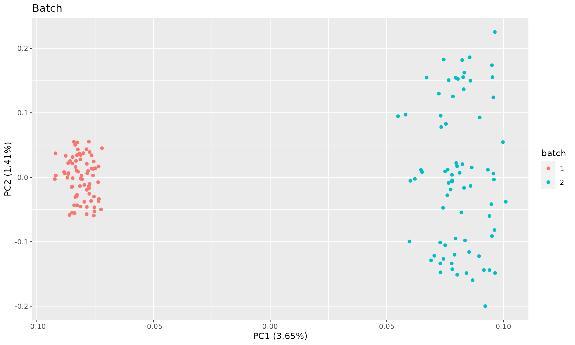
Plot of first two components, colored by batch. PCA does not split the count data by clusters.
PCA, Singular Value Decomposition
PCA is computed by an Singular Value Decomposition (svd) of a centered or centered and scaled matrix to compute PCA of the covariance or correlation matrix. SVD can be considered a generalization of eigenvalue decomposition. In eigenvalue decomposition the D matrix is required to be square.
Given a matrix X of dimension n×p, SVD decomposes it to:
\(X = U D V^{t}\)
U,V define the left and right singular values
U and V are square orthogonal: \(UU^{t} = I_{p}\) \(VV^{t} = I_{n}\)
the paramters nu, nv define the number of left and right singular values (components). The output d is a vector of singular values. See the PCA tutorial for more information.
## $d
## NULL
##
## $u
## [1] 150   2
##
## $v
## [1] 4989    2
This is the exact same as a PCA, if we compare the correlation between the left singular values (150 cells)
##      PC1 PC2
## [1,]   1   0
## [2,]   0   1
Faster Singular Value Decomposition with irlba
The Implicitly restarted Lanczos bidiagonalization algorithm (IRLBA) available in the R package irlba is a fast and memory-efficient way to compute an approximate or partial SVD and it often used in scRNAseq application.It finds a few approximate largest (or, optionally, smallest) singular values and corresponding singular vectors of a sparse or dense matrix using a method of Baglama and Reichel (2005).
When running irlba, you need to define the number of Lanczos iterations (iter) carried out.
## $d
## NULL
##
## $u
## [1] 150   2
##
## $v
## [1] 4989    2
##
## $iter
## NULL
##
## $mprod
## NULL## [,1] [,2]
## [1,] -1 0
## [2,] 0 -1
par(mfrow=c(1,2))
plot(svd1$u[,1], svd2$u[,1], xlab="svd PC1", ylab="irlba, PC1")
plot(svd1$u[,2], svd2$u[,2], xlab="svd PC2", ylab="irlba, PC2")
COA and Pearson residuals
So what does correspondence analysis do and how is it related to decomposition of the Pearson residuals?
As mentioned above a critical step in decomposition is choosing the form of the data that makes more sense. SVD will detect linear vectors that can the most variance in the data. So if the variance is skewed or varies with the mean, it needs normalization.
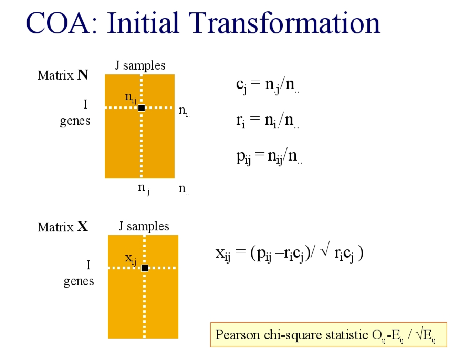
I will describe it in two ways, you could consider the expected value of an element (\(X_{ij}\)) in a matrix N to be the product of its row (\(r_i\)) and column (\(c_j\)) weight, where the row weight is the \(\frac{rowsum}{total sum}\) and thus represents the contribution of that row to the total matrix. Equally, the column weight is the \(\frac{colsum}{total sum}\), and is the contribution of that column to the total. Sometimes the row and column weight are called the row and column mass respectively. The expected weight of every element is the outer product of the row and column weights
In COA, the data are treated like a contingency table so the residuals are the difference between the observed data and the expected, under the assumption that there is no relationship. The Pearson \(\chi^2\) statistic is: \[\frac{observed-expected}{\sqrt{expected}}\] The \(\chi^2\) transformed matrix is then decomposed with SVD.
COA
A much more detailed explanation of correspondence analysis is provided at: https://www.displayr.com/math-correspondence-analysis/
Observed, Expected matrix
The input matrix must be positive count data.
The expected value for each element of the matrix is the product of the row and column weight. This can be easily calculated
rw<-rowSums(mat)/sum(mat) # row weights
cw<-colSums(mat)/sum(mat)  # column weights
expectedValues<- outer(cw, rw)
#dim(expw)
expectedValues[1:2,1:3]
## gene_1 gene_2 gene_3
## cell_1 1.433571e-06 6.881143e-07 4.205143e-07
## cell_2 1.446955e-06 6.945386e-07 4.244403e-07Actual (observed) values
mat[1:3,1:3]## cell_1 cell_2 cell_3
## gene_1 0 0 0
## gene_2 1 0 0
## gene_3 0 0 0Therefore the \(\chi^2\) transformed matrix is just as stated above: \(\frac{observed-expected}{\sqrt{expected}}\)
COA implementations in R
COA has been implement in numberous R packages, including;
ca (ca) CA (FactoMineR) dudi.coa (ade4) cca (vegan) corresp (MASS) ord (made4)
I will compare a few approaches.
COA: the ade4 function. dudi.coa
Correspondence analysis is implemented in ade4 (and made4 extends ade4). The implementation of Correspondence analysis in ade4 is slower than corral (see below), so is not recommended for running COA on scRNAseq. However this is a small dataset, far smaller than a typical scRNAseq data.
The ade4 package provides COA in the function dudi.coa. In the French school, dudi refers to duality diagram (Benzécri, 1973; Holmes, 2008), which is central to the a geometric school of matrix factorization.
## Class: coa dudi
## Call: ade4::dudi.coa(df = mat, scannf = FALSE, nf = 2)
##
## Total inertia: 3.364
##
## Eigenvalues:
##     Ax1     Ax2     Ax3     Ax4     Ax5
## 0.05046 0.04830 0.03039 0.03018 0.02958
##
## Projected inertia (%):
##     Ax1     Ax2     Ax3     Ax4     Ax5
##  1.5003  1.4359  0.9035  0.8972  0.8794
##
## Cumulative projected inertia (%):
##     Ax1   Ax1:2   Ax1:3   Ax1:4   Ax1:5
##   1.500   2.936   3.840   4.737   5.616
##
## (Only 5 dimensions (out of 149) are shown)
The resulting row and column scores and coordinates are in the objects li, co, l1, c1, where l here refers to “lignes” or rows, and c is columns.
coa_ade4$li  #Row coordinates dims =c(4989,10)
coa_ade4$co  #Col coordinates dims=c(150,10)
coa_ade4$l1  #Row scores dims =c(4989,10)
coa_ade4$c1 #Col scores dims=c(150,10)## li l1 co c1
## [1,] 4989 4989 150 150
## [2,] 2 2 2 2
plot(coa_ade4$co[,1], coa_ade4$co[,2], col=pheno$clust, pch=19, xlab="coa_ade4, PC1", ylab="coa_ade4, PC2")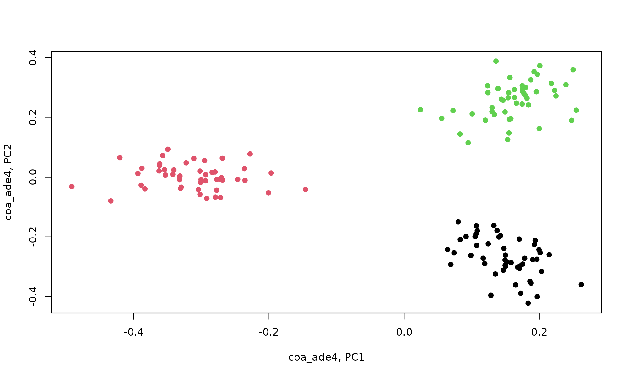
Visualization of results with explor
Results of ade4 matrix factorization can be interactively explored using explor, by default it plots COA results in the biplot, because the features (genes) and cases are on the same scale.
The coordinates are in the object co and it can be seen that COA separates by cell cluster. explor creates plots using scatterD3::scatterD3 which creates interactive scatter plot based on d3.js.
res <- explor::prepare_results(coa_ade4)
explor::CA_var_plot(res, var_hide = "Row", col_var = pheno$clust)
scatterD3::scatterD3(coa_ade4$co[,1], coa_ade4$co[,2], col_var= pheno$clust, ylab = "coa_ade4 PC2", xlab="coa_ade4 PC1")glmPCA- Poisson
Generalized principal component analysis (GLM-PCA), a generalization of PCA to exponential family likelihoods propose Poisson and negative binomial likelihood models (Townes et al., 2019).
glmPCA is iterative, so in this example I will set seed so its reproducible. I discuss about the iterative nature of glmPCA below
set.seed(50)
glmPCA_coa<-glmpca::glmpca(mat,L=2,fam="poi")

dim(glmPCA_coa$factors)  # Column scores dim=c(150,   2)
## [1] 150 2
dim(glmPCA_coa$loadings) # row scoress dim =c(4989 , 2)## [1] 4989 2
plot(glmPCA_coa$factors$dim1, glmPCA_coa$factors$dim2, col=pheno$clust, pch=19, xlab="glmPCA, factors, PC1", ylab="glmPCA, factors, PC2", )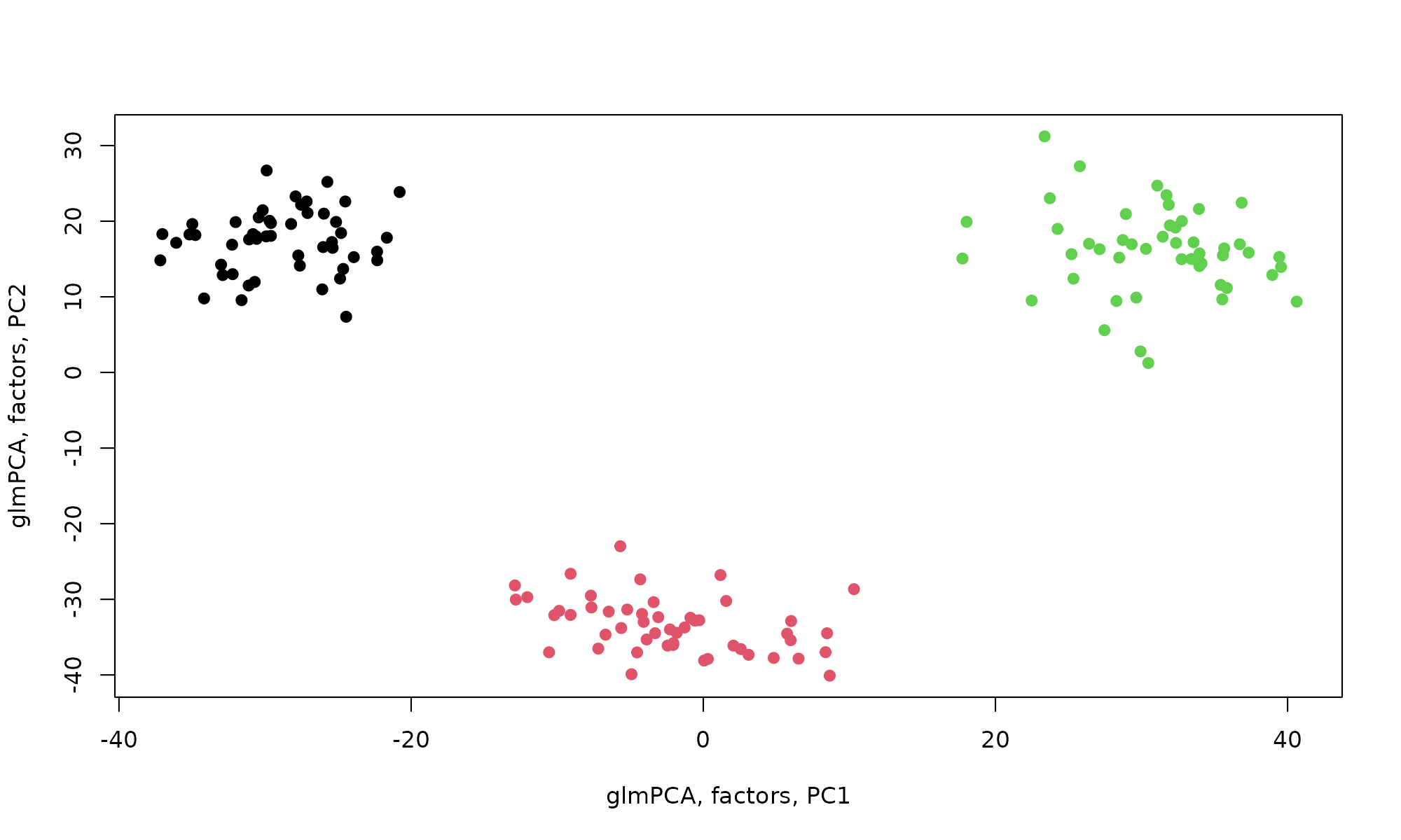
corral
corral from Lauren Hsu uses irlba and sparse matrix representation, providing a fast implementation correspondence analysis in the function corral. corral accepts input formats SingleCellExperiment (Bioconductor), SparseMatrix, matrix, data.frame. See the [dimension reduction vignette]https://www.bioconductor.org/packages/devel/bioc/vignettes/corral/inst/doc/corral_dimred.html from the package for more details.
coa_corral<-corral::corral(mat,ncomp=2)
coa_corral
## corral output summary===========================================
## Output "list" includes standard coordinates (SCu, SCv),
## principal coordinates (PCu, PCv), & SVD output (u, d, v)
## Variance explained----------------------------------------------
## PC1 PC2
## percent.Var.explained 0.02 0.01
## cumulative.Var.explained 0.02 0.03
##
## Dimensions of output elements-----------------------------------
## Singular values (d) :: 2
## Left singular vectors & coordinates (u, SCu, PCu) :: 4989 2
## Right singular vectors & coordinates (v, SCv, PCv) :: 150 2
## See corral help for details on each output element.
## Use plot_embedding to visualize; see docs for details.
## ================================================================
coa_corral$PCu[1:2,] # Row coordinates dims =c(4989,10)## [,1] [,2]
## gene_1 0.6098867 0.6836028
## gene_2 0.1179244 0.2704358
coa_corral$PCv[1:2,] # Col coordinates dims=c(150,10)## [,1] [,2]
## cell_1 -0.2770690 0.007619298
## cell_2 -0.3045123 0.041767103
plot(coa_corral$PCv[,1], coa_corral$PCv[,2], col=pheno$clust, pch=19, xlab="coa corral, PC1", ylab="coa corral, PC2")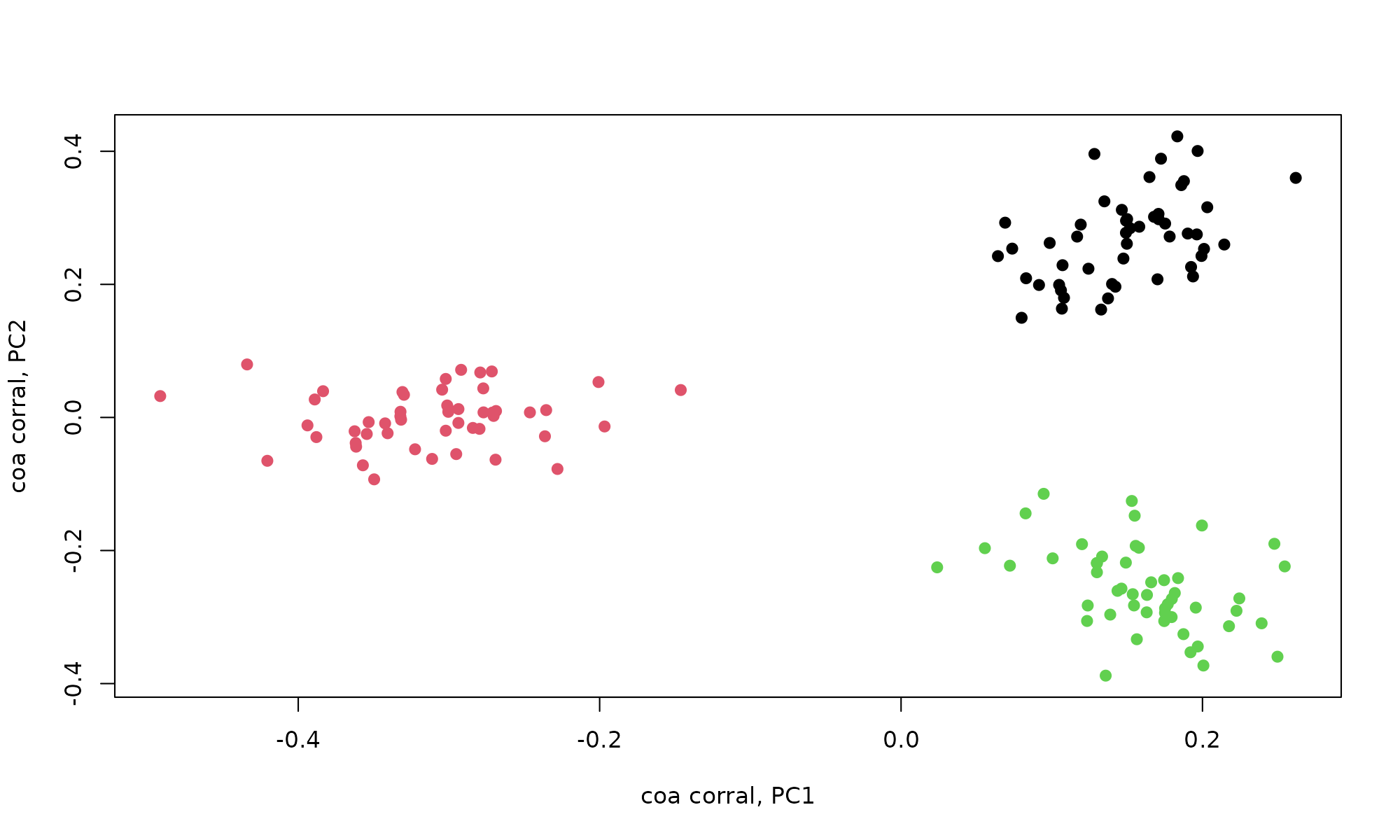
Comparing the output from these COA approaches
Correlation between correspondence analysis and corral is identical
cor(coa_ade4$co[,1], coa_corral$PCv[,1])## [1] 1
cor(coa_ade4$co[,2], coa_corral$PCv[,2])## [1] -1
par(mfrow=c(1,2))
plot(coa_ade4$co[,1], coa_corral$PCv[,1], xlab="coa_ade4, PC1", ylab="coa corral, PC1")
plot(coa_ade4$co[,2], coa_corral$PCv[,2], xlab="coa_ade4, PC2", ylab="coa corral, PC2")
Correlation between glmpca and corral. Note the PCs are flipped, PC1 in corral shares r=0.99 correlation with PC2 of glmpca(type = poi).
cor(glmPCA_coa$factors[,1], coa_corral$PCv[,2])## [1] -0.9893969
cor(glmPCA_coa$factors[,2], coa_corral$PCv[,1])## [1] 0.992287
par(mfrow=c(1,2))
plot(-glmPCA_coa$factors[,1], coa_corral$PCv[,2], xlab="glmPCA Poi, PC1", ylab="coa corral, PC2")
plot(glmPCA_coa$factors[,2], coa_corral$PCv[,1], xlab="glmPCA Poi, PC2", ylab="coa corral, PC1")
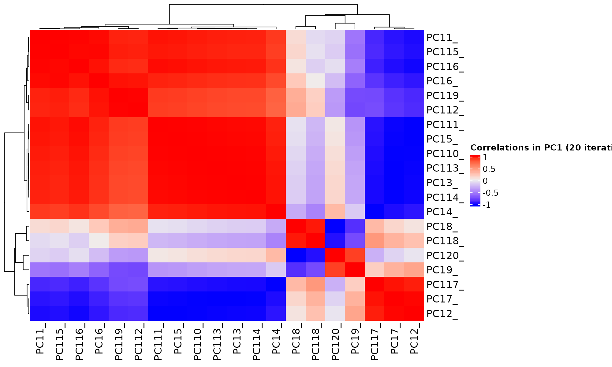
Notes
GLM-PCA provides generalized PCA for probit and logit models but it is an iterative algorithm. Between runs, it tends to flip the order of principal components.
iter=20
tt<-lapply(1:iter, function(x) glmpca::glmpca(mat, L=2, fam="poi"))
factors1<-sapply(1:iter, function(i) tt[[i]]$factors$dim1)  # first factor
factors2<-sapply(1:iter, function(i) tt[[i]]$factors$dim2)  # Second factor

colnames(factors1) = paste0("PC1", 1:iter, sep="_")
colnames(factors2) = paste0("PC2", 1:iter, sep="_")
boxplot(factors1, ylab="factor PC1", xlab="iter", las=2, main="The First PC1 in 20 iterations") # dim=c(150 , iter)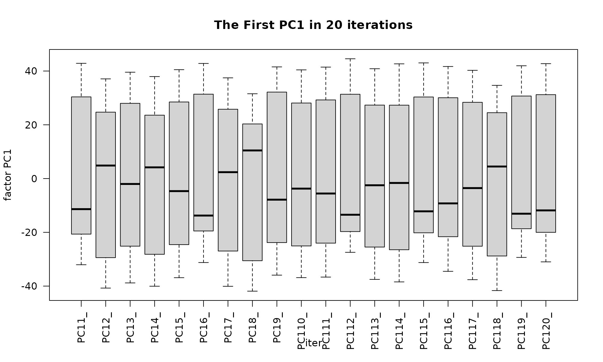
## R version 4.1.0 (2021-05-18)
## Platform: x86_64-pc-linux-gnu (64-bit)
## Running under: Ubuntu 20.04.2 LTS
##
## Matrix products: default
## BLAS/LAPACK: /usr/lib/x86_64-linux-gnu/openblas-pthread/libopenblasp-r0.3.8.so
##
## locale:
##  [1] LC_CTYPE=en_US.UTF-8       LC_NUMERIC=C
##  [3] LC_TIME=en_US.UTF-8        LC_COLLATE=en_US.UTF-8
##  [5] LC_MONETARY=en_US.UTF-8    LC_MESSAGES=C
##  [7] LC_PAPER=en_US.UTF-8       LC_NAME=C
##  [9] LC_ADDRESS=C               LC_TELEPHONE=C
## [11] LC_MEASUREMENT=en_US.UTF-8 LC_IDENTIFICATION=C
##
## attached base packages:
## [1] grid      stats     graphics  grDevices utils     datasets  methods
## [8] base
##
## other attached packages:
##  [1] ComplexHeatmap_2.9.3 scatterD3_1.0.0      glmpca_0.2.0
##  [4] irlba_2.3.3          Matrix_1.3-4         ade4_1.7-17
##  [7] corral_1.3.1         ggfortify_0.4.12     ggplot2_3.3.5
## [10] knitr_1.33
##
## loaded via a namespace (and not attached):
##  [1] bitops_1.0-7                matrixStats_0.60.0
##  [3] fs_1.5.0                    RColorBrewer_1.1-2
##  [5] doParallel_1.0.16           rprojroot_2.0.2
##  [7] GenomeInfoDb_1.29.3         tools_4.1.0
##  [9] bslib_0.2.5.1               utf8_1.2.2
## [11] R6_2.5.0                    DBI_1.1.1
## [13] BiocGenerics_0.39.1         colorspace_2.0-2
## [15] GetoptLong_1.0.5            withr_2.4.2
## [17] tidyselect_1.1.1            gridExtra_2.3
## [19] compiler_4.1.0              textshaping_0.3.5
## [21] Biobase_2.53.0              desc_1.3.0
## [23] DelayedArray_0.19.1         labeling_0.4.2
## [25] sass_0.4.0                  scales_1.1.1
## [27] pkgdown_1.6.1               systemfonts_1.0.2
## [29] stringr_1.4.0               digest_0.6.27
## [31] rmarkdown_2.9               XVector_0.33.0
## [33] dichromat_2.0-0             pkgconfig_2.0.3
## [35] htmltools_0.5.1.1           MatrixGenerics_1.5.2
## [37] highr_0.9                   fastmap_1.1.0
## [39] maps_3.3.0                  GlobalOptions_0.1.2
## [41] htmlwidgets_1.5.3           rlang_0.4.11
## [43] ggthemes_4.2.4              pals_1.7
## [45] farver_2.1.0                shape_1.4.6
## [47] jquerylib_0.1.4             generics_0.1.0
## [49] jsonlite_1.7.2              dplyr_1.0.7
## [51] RCurl_1.98-1.3              magrittr_2.0.1
## [53] GenomeInfoDbData_1.2.6      transport_0.12-2
## [55] Rcpp_1.0.7                  munsell_0.5.0
## [57] S4Vectors_0.31.0            fansi_0.5.0
## [59] lifecycle_1.0.0             stringi_1.7.3
## [61] yaml_2.2.1                  MASS_7.3-54
## [63] SummarizedExperiment_1.23.1 zlibbioc_1.39.0
## [65] parallel_4.1.0              crayon_1.4.1
## [67] lattice_0.20-44             circlize_0.4.13
## [69] mapproj_1.2.7               magick_2.7.2
## [71] pillar_1.6.2                GenomicRanges_1.45.0
## [73] rjson_0.2.20                codetools_0.2-18
## [75] stats4_4.1.0                glue_1.4.2
## [77] evaluate_0.14               data.table_1.14.0
## [79] MultiAssayExperiment_1.19.5 png_0.1-7
## [81] vctrs_0.3.8                 foreach_1.5.1
## [83] gtable_0.3.0                purrr_0.3.4
## [85] tidyr_1.1.3                 clue_0.3-59
## [87] assertthat_0.2.1            cachem_1.0.5
## [89] xfun_0.24                   ragg_1.1.3
## [91] SingleCellExperiment_1.15.1 tibble_3.1.3
## [93] iterators_1.0.13            memoise_2.0.0
## [95] IRanges_2.27.0              ellipse_0.4.2
## [97] cluster_2.1.2               ellipsis_0.3.2
References
Abdi, H., & Valentin, D. (2007). Multiple Correspondence Analysis. In N. Salkind (Ed.), Encyclopedia of Measurement and Statistics (pp. 652–657). Sage Publications, Inc. https://doi.org/10.4135/9781412952644.n299
Baglama, James, and Lothar Reichel. “Augmented implicitly restarted Lanczos bidiagonalization methods.” SIAM Journal on Scientific Computing 27.1 (2005): 19-42.
Benzécri, J.-P. (Ed.). (1973). L’analyse des données.
Busold, C. H., Winter, S., Hauser, N., Bauer, A., Dippon, J., Hoheisel, J. D., & Fellenberg, K. (2005). Integration of GO annotations in Correspondence Analysis: Facilitating the interpretation of microarray data. Bioinformatics, 21(10), 2424–2429. https://doi.org/10.1093/bioinformatics/bti367
Culhane, A C, Perrière, G., & Higgins, D. G. (2003). Cross-platform comparison and visualisation of gene expression data using co-inertia analysis. BMC Bioinformatics, 4(1), 59. https://doi.org/10.1186/1471-2105- 4-59
Culhane, A. C., Perriere, G., Considine, E. C., Cotter, T. G., & Higgins, D. G. (2002). Between-group analysis of microarray data. Bioinformatics, 18(12), 1600–1608. https://doi.org/10.1093/bioinformatics/18.12.1600
Duò, A., Robinson, M. D., & Soneson, C. (2018). A systematic performance evaluation of clustering methods for single cell RNA-seq data. F1000Research, 7, 1141. https://doi.org/10.12688/f1000research.15666.2
Fellenberg, K., Hauser, N. C., Brors, B., Neutzner, A., Hoheisel, J. D., & Vingron, M. (2001). Correspondence analysis applied to microarray data. Proceedings of the National Academy of Sciences, 98(19), 10781–10786. https://doi.org/10.1073/pnas.181597298
Grantham, R., Gautier, C., & Gouy, M. (1980). Codon frequencies in 119 individual genes confirm corsistent choices of degenerate bases according to genome type. Nucleic Acids Research, 8(9), 1893–1912. https://doi.org/10.1093/nar/8.9.1893
Greenacre, M. (2013). The contributions of rare objects in correspondence analysis. Ecology, 94(1), 241–249. https://doi.org/10.1890/11-1730.1
Greenacre, M. J. (1984). Theory and applications of correspondence analysis. Academic Press.
Greenacre, M. J. (2010). Correspondence analysis: Correspondence analysis. Wiley Interdisciplinary Reviews: Computational Statistics, 2(5), 613–619. https://doi.org/10.1002/wics.114
Greenacre, M., & Hastie, T. (1987). The Geometric Interpretation of Correspondence Analysis. Journal of the American Statistical Association, 82(398), 437–447.https://doi.org/10.1080/01621459.1987.10478446
Hafemeister, C., & Satija, R. (2019). Normalization and variance stabilization of single-cell RNA-seq data using regularized negative binomial regression. Genome Biology, 20(1), 296. https://doi.org/10.1186/s13059-019-1874-1
Hicks, S. C., Townes, F. W., Teng, M., & Irizarry, R. A. (2018). Missing data and technical variability in single-cell RNAsequencing experiments. Biostatistics, 19(4), 562–578. https://doi.org/10.1093/biostatistics/kxx053
Hirschfeld, H. O. (1935). A Connection between Correlation and Contingency. Mathematical Proceedings of the Cambridge Philosophical Society, 31(4), 520–524. https://doi.org/10.1017/S0305004100013517
Holmes, S. (2008). Multivariate data analysis: The French way. ArXiv:0805.2879 [Stat], 219–233. https://doi.org/10.1214/193940307000000455
Hsu L, Culhane A. Impact of Data Preprocessing on Integrative Matrix Factorization of Single Cell Data. Front Oncol. 2020;10:973. doi:10.3389/fonc.2020.00973.
Hubert, L., & Arabie, P. (1985). Comparing partitions. Journal of Classification, 2(1), 193–218. https://doi.org/10.1007/BF01908075
Legendre, P., Legendre, L., Legendre, L., & Legendre, L. (1998). Numerical ecology (2nd English ed). Elsevier.
Meng, C., Kuster, B., Culhane, A. C., & Gholami, A. (2014). A multivariate approach to the integration of multi-omics datasets. BMC Bioinformatics, 15(1), 162. https://doi.org/10.1186/1471-2105-15-162
Meng, C., Zeleznik, O. A., Thallinger, G. G., Kuster, B., Gholami, A. M., & Culhane, A. C. (2016). Dimension reduction techniques for the integrative analysis of multi-omics data. Briefings in Bioinformatics, 17(4), 628–641. https://doi.org/10.1093/bib/bbv108
Townes, F.W., Hicks, S.C., Aryee, M.J. et al. Feature selection and dimension reduction for single-cell RNA-Seq based on a multinomial model. Genome Biol 20, 295 (2019). https://doi.org/10.1186/s13059-019-1861-6